astronomix - differentiable mhd for astrophysics in JAX

astronomix (formerly jf1uids) is a differentiable hydrodynamics and magnetohydrodynamics code written in JAX with a focus on astrophysical applications. astronomix is easy to use, well-suited for fast method development, scales to multiple GPUs and its differentiability opens the door for gradient-based inverse modeling and sampling as well as surrogate / solver-in-the-loop training.

Features

• 1D, 2D and 3D hydrodynamics and magnetohydrodynamics simulations scaling to multiple GPUs
• a 5th order finite difference constrained transport WENO MHD scheme following HOW-MHD by Seo & Ryu 2023 as well as the provably divergence free and provably positivity preserving finite volume approach of Pang and Wu (2024) (the WENO scheme is also available standalone for hydrodynamics)
• isothermal hydrodynamics and magnetohydrodynamics are also supported (currently only in the finite difference scheme)
• for finite volume simulations the basic Lax-Friedrichs, HLL and HLLC Riemann solvers as well as the HLLC-LM (Fleischmann et al., 2020) and HYBRID-HLLC & AM-HLLC (Hu et al., 2025) (sequels to HLLC-LM) variants
• novel (possibly) conservative self gravity scheme, with improved stability at strong discontinuities
• spherically symmetric simulations such that mass and energy are conserved based on the scheme of Crittenden and Balachandar (2018)
• backwards and forwards differentiable with adaptive timestepping
• turbulent driving, simple stellar wind, simple radiative cooling modules
• easily extensible, all code is open source

Contents

• Installation
• Hello World! Your first astronomix simulation
• Notebooks for Getting Started
• Showcase
• Scaling tests
• Documentation
• Methodology
• Limitations
• Citing astronomix

Installation

astronomix can be installed via pip

pip install astronomix

Note that if JAX is not yet installed, only the CPU version of JAX will be installed as a dependency. For a GPU-compatible installation of JAX, please refer to the JAX installation guide.

Hello World! Your first astronomix simulation

Below is a minimal example of a 1D hydrodynamics shock tube simulation using astronomix.

import jax.numpy as jnp
from astronomix import (
    SimulationConfig, SimulationParams,
    get_helper_data, finalize_config,
    get_registered_variables, construct_primitive_state,
    time_integration
)

# the SimulationConfig holds static 
# configuration parameters
config = SimulationConfig(
    box_size = 1.0,
    num_cells = 101,
    progress_bar = True
)

# the SimulationParams can be changed
# without causing re-compilation
params = SimulationParams(
    t_end = 0.2,
)

# the variable registry allows for the principled
# access of simulation variables from the state array
registered_variables = get_registered_variables(config)

# next we set up the initial state using the helper data
helper_data = get_helper_data(config)
shock_pos = 0.5
r = helper_data.geometric_centers
rho = jnp.where(r < shock_pos, 1.0, 0.125)
u = jnp.zeros_like(r)
p = jnp.where(r < shock_pos, 1.0, 0.1)

# get initial state
initial_state = construct_primitive_state(
    config = config,
    registered_variables = registered_variables,
    density = rho,
    velocity_x = u,
    gas_pressure = p,
)

# finalize and check the config
config = finalize_config(config, initial_state.shape)

# now we run the simulation
final_state = time_integration(initial_state, config, params, registered_variables)

# the final_state holds the final primitive state, the 
# variables can be accessed via the registered_variables
rho_final = final_state[registered_variables.density_index]
u_final = final_state[registered_variables.velocity_index]
p_final = final_state[registered_variables.pressure_index]

You've just run your first astronomix simulation! You can continue with the notebooks below and we have also prepared a more advanced use-case (stellar wind in driven MHD tubulence) which you can .

Notebooks for Getting Started

• hydrodynamics
  • 1d shock tube
  • 1d spherical check of conservational properties
  • 2d Kelvin-Helmholtz instability
• magnetohydrodynamics
  • 2d Orszag-Tang vortex
  • 3D MHD blast with the 5th order FD scheme
• self-gravity
  • 3d simulation of Evrard's collapse
• stellar wind
  • 1d stellar wind with gradient showcase
  • 1d stellar wind with parameter optimization
  • 3d stellar wind

Showcase

Magnetohydrodynamics simulation with driven turbulence at a resolution of 512³ cells in a fifth order CT MHD scheme run on 4 H200 GPUs.

Magnetohydrodynamics simulation with driven turbulence and stellar wind at a resolution of 512³ cells in a fifth order CT MHD scheme run on 4 H200 GPUs.

Orszag-Tang Vortex	3D Collapse

Gradients Through Stellar Wind

Novel (Possibly) Conservative Self Gravity Scheme, Stable at Strong Discontinuities

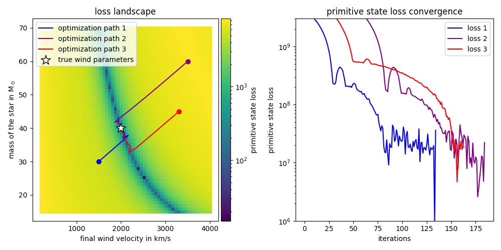
Wind Parameter Optimization

Scaling tests

5th order finite difference vs 2nd order finite volume MHD schemes

Our first scaling tests cover the two MHD schemes implemented in astronomix: the 2nd order finite volume (fv_mhd) scheme and the 5th order finite difference (fd_mhd) scheme.

The following results were obtained on a single NVIDIA H200 GPU, the test run at different resoltions was an MHD blast wave test (see the code).

Runtime benchmarking of the fv_mhd and fd_mhd schemes on a single NVIDIA H200 GPU.

The finite volume scheme is roughly an order of magnitude faster at the same resolution.

But considering the accuracy per computational cost, where we take the 512³ fd_mhd simulation as the reference, the 5th order finite difference scheme is more efficient.

Accuracy versus computational cost for the fv_mhd and fd_mhd schemes on a single NVIDIA H200 GPU.

The finite difference schemes achieves higher accuracy with less computation time.

Multi-GPU scaling

We have tested the multi-GPU scaling of the 5th order finite difference MHD scheme, comparing the runtime of the same simulation on 1 and 4 NVIDIA H200 GPUs (strong scaling).

Multi-GPU scaling of the 5th order finite difference MHD scheme on 4 NVIDIA H200 GPUs.

We reach speedups of up to ~3.5x at 512³ resolution on 4 GPUs compared to a single GPU run. At higher resolutions we would expect to eventually reach perfect scaling. The lower speedup at 600³ cells in our test might be due to other processes running on the GPU node at the time of benchmarking as we are using shared cluster resources.

Documentation

See here.

Methodology

For now we will focus on methodological insights. The basics can be found in

• Van Leer (2006) for the basic 2nd order MUSCL finite volume scheme implemented
• Crittenden and Balachandar (2018) for the spherically symmetric simulations
• Pang and Wu (2024) for the 2nd order provably divergence free and provably positivity preserving finite volume MHD scheme following the research line of operator splitting the MHD system into a hydrodynamic and magnetic update step (also see Dao et al, 2024)
• Seo & Ryu (2023) for the 5th order finite difference constrained transport MHD scheme
• Tomida & Stone (2023) for the coupling of self-gravity to the hydrodynamics equations

2nd order finite volume MHD scheme

The first step in the Pang and Wu (2024) scheme is to split the MHD system into a magnetic and hydrodynamic system. Different from their approach, here we motivate the split based on the primitive form of the MHD equations (their reasoning is generally more formal).

Let us start with the MHD equations in primitive form (see Equation Set 2. in Clarke (2015))

$$ \begin{aligned} \frac{\partial \rho}{\partial t} & =-\nabla \cdot(\rho \vec{v}) \ \frac{\partial \vec{v}}{\partial t} & = -(\vec{v} \cdot \nabla) \vec{v} - \frac{1}{\rho} \nabla p +\frac{1}{\rho}(\nabla \times \vec{B}) \times \vec{B} \ \frac{\partial p}{\partial t} & =- \vec{v} \cdot \nabla p -\gamma p \nabla \cdot \vec{v} \ \frac{\partial \vec{B}}{\partial t} & = \vec{\nabla} \times (\underbrace{\vec{v} \times \vec{B}}_{=-\vec{E}}) \end{aligned} $$

Here $\vec{E}$ denotes the electric field (see Clarke (2015) Sec. 5 or Antonsen (2019) for the derivation of this relation for an ideal MHD fluid with zero viscosity and resistivity). In this primitive form, the magnetic field only directly couples to the velocity as we would expect from the Lorentz force.

Let us now split this system into a hydrodynamic part (which we can turn back into the conservative form)

$$ \text{System A} \quad \begin{cases} \frac{\partial \rho}{\partial t} & =-\nabla \cdot(\rho \vec{v}) \ \frac{\partial \vec{v}}{\partial t} & = -(\vec{v} \cdot \nabla) \vec{v} - \frac{1}{\rho} \nabla p\ \frac{\partial p}{\partial t} & =- \vec{v} \cdot \nabla p -\gamma p \nabla \cdot \vec{v} \ \frac{\partial \vec{B}}{\partial t} & = 0 \end{cases} \quad \Longleftrightarrow \quad \begin{cases} \partial_t \rho + \vec{\nabla} \cdot (\rho \vec{v}) = 0 \ \partial_t (\rho \vec{v}) + \vec{\nabla} \cdot (\rho \vec{v}\vec{v}^T + P\mathbf{1}) = 0 \ \partial_t (\rho e) + \vec{\nabla} \cdot \left[(\rho e + P)\vec{v} \right] = 0 \ \frac{\partial \vec{B}}{\partial t} = 0 \end{cases} $$

and a magnetic part

$$ \text{System B} \quad \begin{cases} \frac{\partial \rho}{\partial t} & = 0 \ \frac{\partial \vec{v}}{\partial t} & = \frac{1}{\rho}(\nabla \times \vec{B}) \times \vec{B} \ \frac{\partial p}{\partial t} & = 0 \ \frac{\partial \vec{B}}{\partial t} & = \vec{\nabla} \times (\vec{v} \times \vec{B}) \end{cases} $$

Where for an MHD time-step we apply a second order operator splitting approach

$$ \vec{U}^{n+1} = S_A^{\frac{\Delta t}{2}} \circ S_B^{\Delta t} \circ S_A^{\frac{\Delta t}{2}} \vec{U}^n $$

We solve the hydrodynamical system A as before and for system B we use finite differencing and a fixed-point iteration.

On a grid in three dimensions, the curl of a field $\vec{A} \in \mathbb{R}^3$ is discretized as

$$ \vec{\nabla} \times \vec{A}{i,j,k} := \begin{pmatrix} \frac{A^z{i,j+1,k} - A^z_{i,j-1,k}}{2 \Delta y} - \frac{A^y_{i,j,k+1} - A^y_{i,j,k-1}}{2 \Delta z} \ \frac{A^x_{i,j,k+1} - A^x_{i,j,k-1}}{2 \Delta z} - \frac{A^z_{i+1,j,k} - A^z_{i-1,j,k}}{2 \Delta x} \ \frac{A^y_{i+1,j,k} - A^y_{i-1,j,k}}{2 \Delta x} - \frac{A^x_{i,j+1,k} - A^x_{i,j-1,k}}{2 \Delta y} \end{pmatrix} $$

and on a grid in two dimensions as (the field is still $\vec{A} \in \mathbb{R}^3$)

$$ \vec{\nabla} \times \vec{A}{i,j} := \begin{pmatrix} \frac{A^z{i,j+1} - A^z_{i,j-1}}{2 \Delta y} \ -\frac{A^z_{i+1,j} - A^z_{i-1,j}}{2 \Delta x} \ \frac{A^y_{i+1,j} - A^y_{i-1,j}}{2 \Delta x} - \frac{A^x_{i,j+1} - A^x_{i,j-1}}{2 \Delta y} \end{pmatrix} $$

The central difference divergence in 3D is given as

$$ \vec{\nabla} \cdot \vec{A}{i,j,k} := \frac{A^x{i+1,j,k} - A^x_{i-1,j,k}}{2 \Delta x} + \frac{A^y_{i,j+1,k} - A^y_{i,j-1,k}}{2 \Delta y} + \frac{A^z_{i,j,k+1} - A^z_{i,j,k-1}}{2 \Delta z} $$

and in 2D as

$$ \vec{\nabla} \cdot \vec{A}{i,j} := \frac{A^x{i+1,j} - A^x_{i-1,j}}{2 \Delta x} + \frac{A^y_{i,j+1} - A^y_{i,j-1}}{2 \Delta y} $$

Note that the discrete divergence of a discrete curl as defined above still vanishes. For the 3D field on the 2D grid, this follows from

$$ \begin{gathered} \vec{\nabla} \cdot (\vec{\nabla} \times \vec{A}{i,j}) = \frac{1}{2 \Delta x}\left( \frac{A^z{i+1,j+1} - A^z_{i+1,j-1}}{2 \Delta y} - \frac{A^z_{i-1,j+1} - A^z_{i-1,j-1}}{2 \Delta y} \right) \ + \frac{1}{2 \Delta y}\left( -\frac{A^z_{i+1,j+1} - A^z_{i-1,j+1}}{2 \Delta x} + \frac{A^z_{i+1,j-1} - A^z_{i-1,j-1}}{2 \Delta x} \right) \ = \frac{1}{4 \Delta y \Delta x}\big(A^z_{i+1,j+1} - A^z_{i+1,j+1} + A^z_{i+1,j-1} - A^z_{i+1,j-1} \ + A^z_{i-1,j+1} - A^z_{i-1,j+1} + A^z_{i-1,j-1} - A^z_{i-1,j-1} \big) \ = 0 \end{gathered} $$

We perform a time-step of System B given by

$$ \partial_t \begin{pmatrix} \vec{v} \ \vec{B} \end{pmatrix} = \begin{pmatrix} \frac{1}{\rho}(\nabla \times \vec{B}) \times \vec{B} \ \vec{\nabla} \times (\vec{v} \times \vec{B}) \end{pmatrix} =: \vec{\Psi}\left(\begin{pmatrix} \vec{v} \ \vec{B} \end{pmatrix}\right) $$

using an implicit midpoint method

$$ \vec{R}^{(n+1)} = \vec{R}^{(n)} + \Delta t , \vec{\Psi}\left(\frac{1}{2}\left( \vec{R}^{(n)} + \vec{R}^{(n + 1)} \right) \right) $$

with

$$ \vec{R} = \begin{pmatrix} \vec{v} \ \vec{B} \end{pmatrix} $$

We solve this implicit equation using a fixed-point iteration

$$ \begin{gathered} \vec{R}^{(0)} = \vec{R}^{(n)}, \ \vec{R}^{(k+1)} = \vec{R}^{(n)} + \Delta t, \vec{\Psi}!\left( \frac{\vec{R}^{(n)} + \vec{R}^{(k)}}{2} \right), \quad k = 0, 1, \dots, \ \text{until }; \max\Big( \left| \vec{B}^{(k+1)} - \vec{B}^{(k)} \right|{\infty}, \left| \vec{v}^{(k+1)} - \vec{v}^{(k)} \right|{\infty} \Big) < \varepsilon_{\mathrm{tol}} \end{gathered} $$

We use $\varepsilon_{\mathrm{tol}} = 10^{-10}$ in double precision and $\varepsilon_{\mathrm{tol}} = 10^{-5}$ in single precision.

This iteration usually converges in a few ($5$ to $9$) iterations (Pang and Wu, 2024) and thus is relatively inexpensive. Here we leave extensive performance profiling for future work. Note that all our updates to the magnetic field are numerical curls of vector fields, we therefore never add divergence to the magnetic field and retain $\vec{\nabla} \cdot \vec{B} = 0$ by design.

For the provably positivity preserving property of the hydrodynamic update, we refer to Pang and Wu (2024).

Artificial oscillations in the fv_mhd scheme in 3D with HLL/HLLC Riemann solvers

In Pang and Wu (2024) the positivity preserving property is obtained based on using a Lax-Friedrichs Riemann flux combined with a specific limiting procedure. For our turbulence simulations we would like to use a less dissipative Riemann solver. In our 2D tests, using HLL or HLLC worked well without problems.

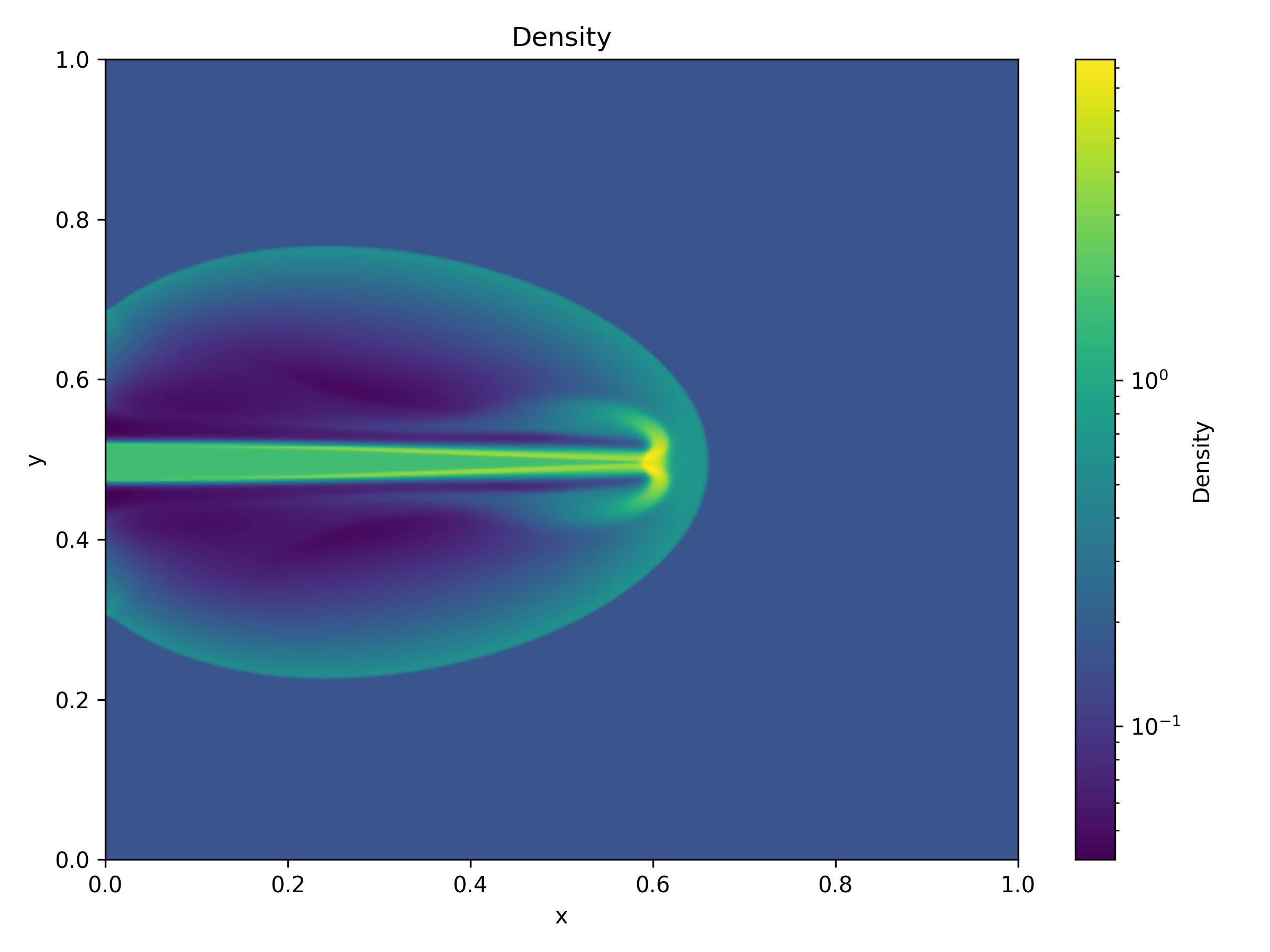
MHD jet simulated with the fv_mhd scheme.

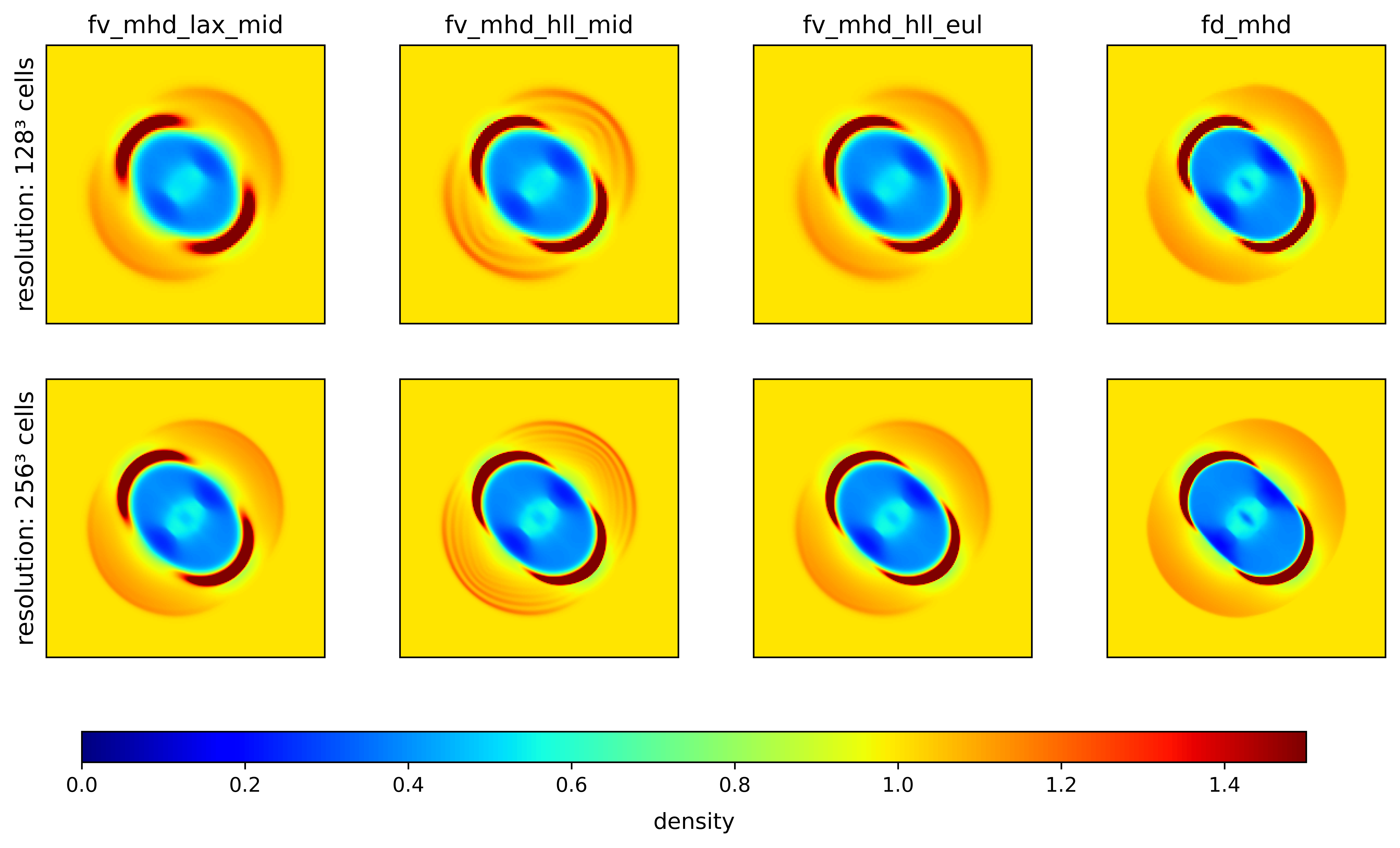
However, in 3D we observed the development of artificial oscillations scaling with the grid scale. These oscillations could be mitigated by using a first order implicit Euler solve for the magnetic update step instead of the implicit midpoint method.

The less dissipative HLL Riemann solver combined with the implicit midpoint magnetic update produces numerical oscillations.

Boundary conditions in the finite volume scheme

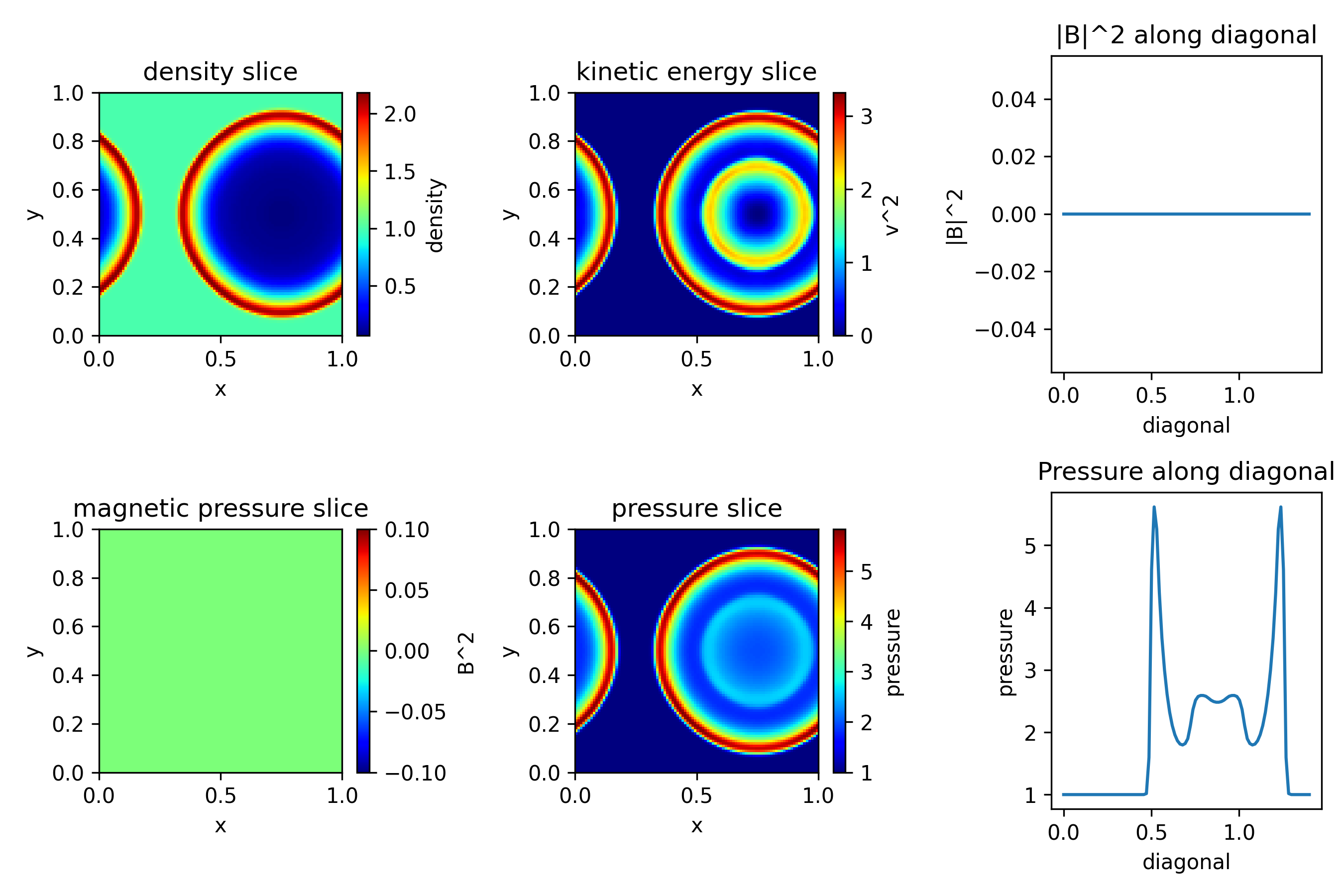
In the finite volume scheme, boundary conditions are applied based on ghost cells. Periodic boundary conditions as well as "open boundaries" and reflective boundaries are supported. Note that 'open boundaries' here refers to van Neumann zero gradient boundary conditions, i.e. the ghost cells are filled with the values of the outermost cells in the physical domain. In settings where not all of the characteristics are outgoing at the boundary, this can lead to artefacts caused by the boundary. An example of such artefacts is illustrated below.

Periodic boundary conditions.

Van Neumann zero gradient boundary conditions.

Coupling self-gravity to the hydrodynamics equations

We have developed a new self-gravity scheme for FD simulations, to be described here soon.

A simple source-term scheme - energy is not conserved

Consider the gravitational potential $\Phi_i$ to be already calculated on the cell centers (cell $i$). By the central difference

$$ g_i = -\frac{\Phi_{i+1} - \Phi_{i-1}}{2 \Delta x} $$

we can approximate the acceleration on the gas in the $i$-th cell.

The simplest source-term coupling of the potential to the hydrodynamics is by an update

$$ \vec{U}_i \leftarrow \vec{U}_i + \Delta t \vec{S}_i, \quad \vec{S}_i = \begin{pmatrix} 0 \ \rho g_i \ \rho v_i g_i \end{pmatrix} $$

where $\Delta t$ is the hydro-timestep. This update closely follows the Euler gravity equation.

However, this scheme does not conserve energy, essentially because the mass actually transported in the field is not the bulk flux $\rho v_i$ but the Riemann flux. When we for instance consider the HLLC flux in the central formulation:

$$ \vec{F}{\ast} = \underbrace{\tfrac{1}{2}\left(\vec{F}{L} + \vec{F}{R}\right)}{\text{bulk-flux component}} + \underbrace{\tfrac{1}{2}\left[ S_{L}\left(\vec{U}{\ast L}-\vec{U}{L}\right) + | S_{\ast} | \left(\vec{U}{\ast L}-\vec{U}{\ast R}\right) + S_{R}\left(\vec{U}{\ast R}-\vec{U}{R}\right) \right]}_{\text{gradient-based component}} $$

we can see a bulk-flux component and a gradient-based component. The higher the resolution, the more aligned will the Riemann flux and bulk flux be, becoming equal for $\Delta x \rightarrow 0$. We therefore expect better conservational properties at higher spatial resolution.

For a spherical collapse test (Evrard's collapse)

$$ \rho(r)= \begin{cases}M /\left(2 \pi R^2 r\right) & \text { for } r \leq R \ 0 & \text { for } r>R .\end{cases}, \quad M = 1, R = 1, G = 1 $$

the results of the simple source-term scheme are presented below. The results of our (near-)energy-conserving scheme are also shown in the figure.

Energy conservation properties of the simple source-term scheme (non-conservative) and our scheme (conservative) (described later on).

As expected, the total energy is not conserved with the error improving at higher resolution. Note that the energy error is first order in time, so taking smaller time steps does not help (Springel, 2010).

A (near-)energy-conserving but potentially unstable source-term scheme

We will now consider the source-term scheme as implemented in ATHENA (implemented here) and described in Tomida et al. (2023, Sec. 3.2.3), which draws from but is not identical to the fully conservative scheme of Mullen et al. (2021).

In addition to the central difference acceleration we also calculate approximations for accelerations at the interfaces as

$$ g_{i-\frac{1}{2}} = -\frac{\Phi_{i} - \Phi_{i-1}}{\Delta x}, \quad g_{i+\frac{1}{2}} = -\frac{\Phi_{i+1} - \Phi_{i}}{\Delta x} $$

and in the energy source-term use the Riemann fluxes

$$ \vec{U}i \leftarrow \vec{U}i + \Delta t \vec{S}i, \quad \vec{S}i = \begin{pmatrix} 0 \ \rho g_i \ \frac{1}{2}\left((\rho v){i-\frac{1}{2}}^\text{Riemann} g{i-\frac{1}{2}} + (\rho v){i+\frac{1}{2}}^\text{Riemann} g{i+\frac{1}{2}}\right) \end{pmatrix} $$

In my view, this scheme has the following flaws:

• The momentum and energy update become misaligned, while this might have a positive corrective effect in some cases, in others we will make unwanted changes to the internal energy.
• Consider adjacent cells $i$ and $i+1$, each cell receives a term $\frac{1}{2} \rho v_{i+\frac{1}{2}}^\text{Riemann} g_{i+\frac{1}{2}}$ added, these terms correspond to the Riemann flux through the interface at $x_{i+\tfrac{1}{2}}$ which brings about the improved energy conservation (the energy source term reflects the mass actually moved in the potential); however, the half-half split of the Riemann flux between adjacent cells can be problematic: consider a discontinuity where one of the adjacent cells has very little energy to begin with and the flux flows against the potential - the half-half split means that we consider half of the work done against the potential to be done by the energy-depleted cell.

I assume the second aspect to be the reason why this scheme failed for Evrard's collapse in my tests, producing negative pressures at the discontinuity.

Failure mode of the half-half-split scheme compared to our riemann-split scheme

This is substantiated by the observation that our improved scheme, which replaces the half-half split, can simulate Evrard's collapse successfully.

Our (near-)energy-conserving scheme

This is very much work in progress but the main idea is to replace the half-half split.

Consider the interface between cells $i$ and $i+1$. In the half-half split scheme, both cells receive an energy source term $\frac{1}{2} \rho v_{i+\frac{1}{2}}^\text{Riemann} g_{i+\frac{1}{2}}$.

Now, consider that we can write the Riemann flux as

$$ F^\text{Riemann}{i+\frac{1}{2}} = \frac{1}{2}\left( F_L + F_R \right) + F\text{diffusive} $$

where $F_L$ and $F_R$ are the bulk fluxes from the left and right state. We might split the Riemann flux into

$$ F^\text{Riemann}{i+\frac{1}{2}} = \underbrace{\frac{1}{2} F_L + \max(F\text{diffusive}, 0)}{\text{cell $i$ accounts for this}} + \underbrace{\frac{1}{2} F_R + \min(F\text{diffusive}, 0)}_{\text{cell $i+1$ accounts for this}} $$

For a piecewise constant reconstruction $F_L = F_i$ and $F_R = F_{i+1}$ (bulk fluxes $F_i$ and $F_{i+1}$) for the interface between cells $i$ and $i+1$. Similarly $F_L = F_{i-1}$ and $F_R = F_{i}$ for the interface between cells $i-1$ and $i$. For the case of $g_{i+\tfrac{1}{2}} = g_{i-\tfrac{1}{2}} = g_i$ and $F_\text{diffusive} = 0$ we recover the simple (non-conservative) source-term scheme. Therefore our scheme can be seen as a correction to the simple source-term scheme.

More on this will be presented in future work.

Limitations

The finite difference MHD scheme was recently implemented and currently only supports periodic boundary conditions. Currently, cosmic rays not supported with the finite difference scheme. The finite difference MHD scheme is very unstable for zero-magnetic fields (to be improved), do not activate MHD if you have zero magnetic fields.

Citing astronomix

If you use astronomix in your research, please cite via

@misc{storcks_astronomix_2025,
  doi = {10.5281/ZENODO.17782162},
  url = {https://zenodo.org/doi/10.5281/zenodo.17782162},
  author = {Storcks, Leonard},
  title = {astronomix - differentiable MHD in JAX},
  publisher = {Zenodo},
  year = {2025},
  copyright = {MIT License}
}

There is also a workshop paper on an earlier stage of the project:

Storcks, L., & Buck, T. (2024). Differentiable Conservative Radially Symmetric Fluid Simulations and Stellar Winds--jf1uids. arXiv preprint arXiv:2410.23093.